Introduction to Active Contour Model
Mingqi Gao
Image Segmentation plays a significant role in the field of image analyzing. To obtain accurate segmentation results, several methods have been proposed, like clustering methods, graph-based methods and learning-based methods et al. In this post, a different model is introduced, named Active Contour Model, which segments input image by evolving a smooth curve (active contour) iteratively. Relevant code can be found at the end of this page.
Note: if you have trouble seeing the following mathematical formulas and figures, try refreshing this page. If the error persists, please let me know via email.
1. What is Active Contour Model
Active Contour Model (ACM) is an iterative model for image segmentation, whose basic idea is that the object boundary is represented as a close and smooth curve (active contour), can be obtained by evolving an initial curve under the guidance of the input image information.
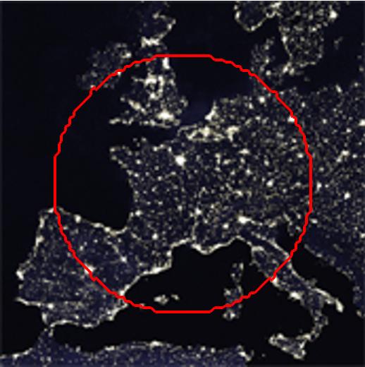
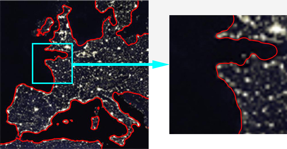
Figure 1. Segmentation result obtained using active contour model. Left: the given image with initial contour (red circle); Middle: the iterative segmentation process; Right: locally enlarged segmentation result.
The figure above illustrates how active contour model works by taking an example of segmenting the image of Europe night-lights. It can be seen that after several iterations, the object in the given image is enclosed by the closed and smooth curve.
Up to now there have been a large number of published active contour models, which are mainly divided into 2 categories: Edge-based ACMs and Region-based ACMs according to the image information they use. Edge-based models are based on an assumption that the image information nears the object boundary changes sharply. In terms of Region-based models, they utilize a certain region descriptor (like intensity, color or texture) to depict the image information of different regions, handling the motion of acitve contours by homogenizing the descriptors in each region.
2. Why Active Contours
Compared with other segmentation models, there are two main advantages ACMs have:
In ACMs, the segmentation result of given image is encircled by closed and smooth curve, which is able to perfectly describe the object boundary and obtain sub-pixel segmentation accuracy.
Generally, due to the evolving curve is implicitly expressed through level set function, making ACMs numerially stable during the iteration. In addition, the topological changes of objects to be segmented can be achieved.
3. Chan-Vese Model
In practice, there are few edge-based models that can achieve desired segmentation results, because of the presence of image noise and discontinuous boundaries with strong gradients in real scene. Thus region-based models have been widely studied so far. Here the region-based model is demonstrated by giving an example of a well-known and typical segmentation mehtod: Chan-Vese Model.
Before discussing the concrete form of Chan-Vese Model, we define subset $\Omega \subset {\mathbb{R}^2}$ as the image field, ${u_0}:\Omega \to \mathbb{R}$ as the given image. Let $C$ in $\Omega$ express the evolving curve, as the boundary of the open subset $\omega \subset \Omega$, and thus we can defind the region $inside(C)$ and $outside(C)$ as $\omega$ and $\Omega \backslash \omega$ respectively.
3.1 Energy functional definition
In the model proposed by Chan and Vese, to generalize the segmentation problem, they assume that the given image is formed by 2 regions with homogeneous intensity. Thus $u_0$ can be approximately expressed as: $${u_0}(x,y) = \begin{cases} {u_0}^{obj}, & \text{if}\ (x,y) \in object\ region \\\\\\ {u_0}^{bk}, & \text{if}\ (x,y) \in background\ region \end{cases}$$ Under this assumption, for the evolving curve $C$ at any time, a fitting term can be solved to assess the macthing degree between $C$ and real object boundary: $$ \begin{align} F_1(C)+F_2(C)&= \int_{inside(C)} {|{u_0}(x,y) - {c_1}{|^2}dxdy} \\&+ \int_{outside(C)} {|{u_0}(x,y) - {c_2}{|^2}dxdy} \end{align} $$ where $c_1$, $c_2$ are the average intensities of $inside(C)$ and $outside(C)$, respectively. From the formula above, it is clear that the value of $F_1(C)+F_2(C)$ reaches its minimum ($\approx 0$)only when $C$ converges to the object boundary.
Therefore, this model converted the problem of image segmentation into a minimization problem, in which the segmentation result can be achieved by iteratively evolving $C$. In order to smooth the segmentation result, the regularized terms penalizing the length of $C$ and the area of $\omega$ have been considered and thus, the integrated energy functional is formulated as: $$ \begin{align} \mathcal{F}^{CV}(c_1 ,{c_2},{C})&=\mu \cdot Length(C) + \nu \cdot Area(inside(C))\\&+ \lambda_1 \cdot \int_{inside(C)} {|{u_0}(x,y) - {c_1}{|^2}dxdy} \\&+ \lambda_2 \cdot \int_{outside(C)} {|{u_0}(x,y) - {c_2}{|^2}dxdy} \end{align} $$ where $\mu$, $\nu$, $\lambda_1$ and $\lambda_2$ are fixed parameters, to adjust the impact of each term on segmentation result.
3.2 Level set method
Compared with traditional parametric curve, due to the level set method that implicitly expresses active contour can make evolution process numerical stable, and also can handle topological changes more easily, it has been used in most ACMs. Let $\phi: \Omega\to \mathbb{R}$ be the level set function, which is generally defined as the Signed Distance Function (SDF): $$ \phi(x,y) = \begin{cases} 0, & \text{if}\ (x,y) \in C\\ +d(x,y,C), & \text{if}\ (x,y) \in inside(C) \\ -d(x,y,C), & \text{if}\ (x,y) \in outside(C) \end{cases} $$ where $d(x,y,C)$ is the shortest distance between $(x,y)$ and C. The diagram of $\phi$ is showed as follows:
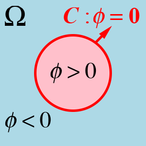
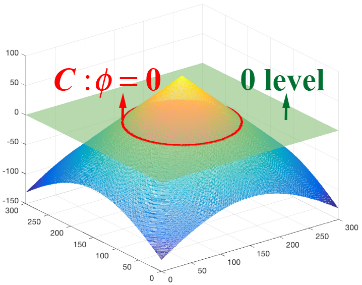
Figure 2. The example of the level set method. Left: The implicit representation of $C$ (red circle) on domain $\Omega$, which is divided into 2 regions according to $\phi$; Right: The 3D visualization of corresponding level set function $\phi$.
To distinguish $inside(C)$ and $outside(C)$ in $\Omega$, Heaviside function $H(z)$ is integrated into the energy functional, defined as follow: $$ H(z) = \begin{cases} 1, & \text{if}\ z \ge 0\\ 0, & \text{if}\ z<0 \end{cases}, \ H’(z)=\delta(z) $$
In Chan and Vese’s model, to facilitate the computation of Euler–Lagrange equations of level set function $\phi$, they consider slightly regularized versions of the functions $H(z)$ and $\delta (z)$, denoted by ${H_\varepsilon }(z)$ and ${\delta_\varepsilon }(z)$ [1]. As a result, the final energy functional is formulated as: $$ \begin{align} \mathcal{F}^{CV}({c_1},{c_2},\phi ) &=\mu \cdot \int_\Omega {\delta_\varepsilon(\phi (x,y))|\nabla \phi (x,y)|dxdy} \\ &+\nu \cdot \int_\Omega {H_\varepsilon(\phi (x,y))dxdy}\\ &+\lambda_1 \cdot \int_\Omega{ { |{u_0}(x,y) - {c_1}{|^2} \cdot H_\varepsilon(\phi (x,y))}dxdy}\\ &+\lambda_2 \cdot \int_\Omega{ { |{u_0}(x,y) - {c_2}{|^2} \cdot (1-H_\varepsilon(\phi (x,y)))}dxdy} \end{align} $$
With the energy functional, the $\phi$ that implicitly represents the real object boundary can be solved by conducting gradient descent algorithm: $$ { \phi^{t+1} = {\phi^t} + \Delta{t} \cdot \frac{d{\phi^t}}{dt}} $$ where: $$ \begin{align} \frac{ d{\phi^t}}{dt} &= -\frac{ {\partial { \mathcal{F}^{CV}}({c_1},{c_2},{\phi^t})}}{ {\partial {\phi^t}}}\\\ &=\delta_\varepsilon(\phi (x,y)) \cdot [\mu \cdot div(\frac{ {\nabla {\phi^t}}}{ {|\nabla {\phi^t}|}})-\nu-\lambda_1 \cdot (u_0-c_1)^2+\lambda_2 \cdot (u_0-c_2)^2] \end{align} $$ and $\phi _0$ is the level set function representing the initial contour.
3.3 Code available
The code of this model is provided HERE. In traditional Chan-Vese model, to prevent $\phi$ from losing its nature as a SDF during the minimization process, a re-initialization is needed. This process, however, is time-consuming and in turn to decrease the segmentation efficiency. To cope with this problem, I made some improvements to the iteration process by integrating an additional term proposed by Chunming Li et al. [2]: $$ \mathcal {P}(\phi ) = \int_\Omega {\frac{1}{2}{ {(|\nabla \phi (x,y)| - 1)}^2}dxdy} $$
From the term above, it is clear that the point that its gradient is larger than 1 will be penalized during the evolution process. Thus the subsequent re-initialization can be eliminated.
Note: To use it as academic purpose, please cite the following papers:
[1] Active Contours Without Edges, Tony F. Chan and Luminita A. Vese. IEEE Trans on Image Processing, 2001.
[2] Level Set Evolution Without Re-initialization: A New Variational Formulation, Chunming Li, Chenyang Xu, Changfeng Gui, and Martin D. Fox. IEEE CVPR, 2005.