Factorization based Active Contour Model
Mingqi Gao, Hengxin Chen, Shenhai Zheng and Bin Fang
As a sub-problem of image segmentation, texture segmentation also has important research significance. In this blog, the idea of factorization based active contour model (FACM) is provided. Different with other ACMs, Here we integrated a new metric into the energy functional, which can assess the probability that a pixel belongs to each component region more accurately. Relevant code can be found at the end of this page.
Note: if you have trouble seeing the following mathematical formulas and figures, try refreshing this page. If the error persists, please let me know via email.
Method
FACM consists of two terms: a factorization based fitting energy ${\varepsilon _F}$ for distinguishing object and background, and a regularization term ${\varepsilon _R}$ [1] for eliminating re-initialization process. The main procedure of this model are shown as below:
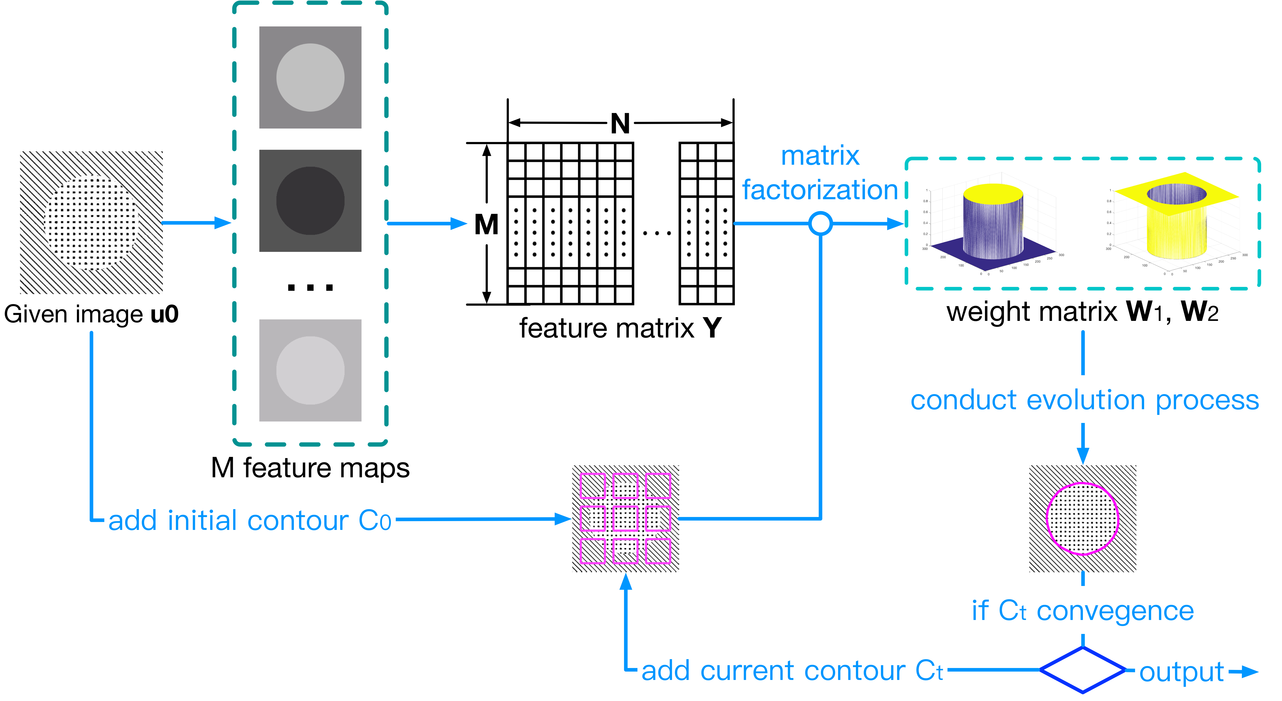
Figure 1. The diagram of FACM. Firstly, the feature matrix is computed over the input image, in which different kinds of texture features are mixed to improve the separability of each region. And then, an initial contour will be given to start the segmentation process. By computing the representative features of each region and their weights at each pixel, the active contour is updated repeatedly until convergence.
To describe the texture information of input image more accurately, we compute the local spectral histogram [2] from the input image $u_0:\Omega \to \mathbb{R}$. Firstly, a set of feature maps will be computed from $u_0$ through convolution. And then, for each pixel $(x,y) \in \Omega$, its spectral histogram is obtained by concatenating several histograms computed over a $w\times w$ window in each feature map: $$\boldsymbol{h} _{w}(x,y)= \left[\ \boldsymbol{h} _{w,1}(x,y)^T \right.,\boldsymbol{h} _{w,2}(x,y)^T,\text{...}\left. {,\boldsymbol{h} _{w,K}(x,y)^T} \right]^T$$
Let $\boldsymbol{h}_w(x,y)$ be an $M\times 1$ vector, we integrate all of which into a $M\times N$ matrix $\mathbf{Y}$ to facilitate the subsequent process, where $N$ denotes the number of pixels in $u_0$. To form a general segmentation model, we assume that $u_0$ consists of 2 regions($\Omega_1 \text{and}\ \Omega_2$) whose texture features are even-distributed. For each pixel in $u_0$, due to its feature histogram is computed accumulatively, which can be regarded as the linear combination of the representative histograms of each region, with the weights ranging from 0 to 1. According to feactorization theory [2], the feature matrix can be decomposed as following form: $$ \mathbf{Y}=\mathbf{R}\times \mathbf{W}+n $$ where $\mathbf{R}=[ \boldsymbol{r}_1, \boldsymbol{r}_2]$ is an $M\times 2$ matrix of representative histograms, containing the average histograms of $\Omega_1$ and $\Omega_2$. $\mathbf{W}$ is a $2\times N$ matrix, containing the weights of two regions in each pixel. $n$ means the additional noise.
In terms of weights, it can be reasoned that for each pixel, the closer it gets to a certain region, the higher weight of corresponding region at this pixel is. Hence we set a fitting term encouraging the weights of $\Omega_1$ and $\Omega_2$ at the pixels within them reach the highest, respectively: $$\begin{align} {\varepsilon_F}(\mathbf{R},\phi ) &=\int_\Omega { {(1- \mathbf{W_1}(x,y))} { H_\varepsilon(\phi (x,y))} dxdy} \\ &+\int_\Omega { {(1- \mathbf{W_2}(x,y))} {(1 - H_\varepsilon(\phi (x,y)))} dxdy} \end{align}$$ where $\mathbf{W}_1$ and $\mathbf{W}_2$ mean two matrices having the same size with $u_0$, referring to the weights of $\Omega_1$ and $\Omega_2$ at each pixel. From the fitting term, it is clear that the value of this term will reach its minimum only when the contour converges to the object boundary. In this equation, different regions are implicitly represented by level set method. For more details about this, please read my former blog.
To solve the weight matrix $\mathbf{W}_1$ and $\mathbf{W}_2$, the least squares method is used: $$\mathbf{W} = [{\boldsymbol{w}_1}^T,{\boldsymbol{w}_2}^T]^T = {(\mathbf{R}{\mathbf{R}^T})^{ - 1}}{\mathbf{R}^T}\mathbf{Y}$$ where $\boldsymbol{w}_1$ and $\boldsymbol{w}_2$ are 2 row vectors. To facilitate the description of the weight of representative features in each pixel, these are converted into two matrices $\mathbf{W}_1$ and $\mathbf{W}_2$. By integrating the regularization term , the final energy functional is defined as below: $$ \begin{align} \mathcal{F}^{FACM}(\mathbf{R},\phi ) &=\mu \cdot \int_\Omega { {(1- \mathbf{W_1}(x,y))} { H_\varepsilon(\phi (x,y))} dxdy} \\ &+\mu \cdot \int_\Omega { {(1- \mathbf{W_2}(x,y))} {(1 - H_\varepsilon(\phi (x,y)))} dxdy}\\ &+ \nu \cdot \int_\Omega {\frac{1}{2}{ {(|\nabla \phi (x,y)| - 1)}^2}dxdy} \end{align} $$ where $\mu$ and $\nu$ are positive parameters adjusting the impact of each energy term on segmentation results. The final object boundary can be achieved by the gradient descent with respect to $\phi$.
Figure 2. The segmentation process of FACM. From left to right: the active contours in different stages when segmenting images with noise, inhomogeneous illumination and complex textures.
From the segmentation results shown above, it is clear that the object boundary can be achieved within very limited iterations, which is mainly attributed to the rich texture features and factorization-based fitting term.
Code available
The code of FACM for texture segmentation is provided HERE.
Note: To use it as academic purpose, please cite the following paper:
A Factorization based Active Contour Model for Texture Segmentation, Mingqi Gao, Hengxin Chen, Shenhai Zheng and Bin Fang. IEEE International Conference on Image Processing (ICIP), 2016.
Main references
[1] Factorization-based texture segmentation, Jiangye Yuan, Deliang Wang, and Anil M Cheriyadat. IEEE Trans on Image Processing (TIP), 2015.
[2] Level Set Evolution Without Re-initialization: A New Variational Formulation, Chunming Li, Chenyang Xu, Changfeng Gui, and Martin D. Fox. IEEE CVPR, 2005.